In this example, each record of an industrial process includes a composition (or run) number, a process type and a final status. The goal is to create a column that will show the order of records with filter criteria based on filter settings. The original table before filtering looks like this.
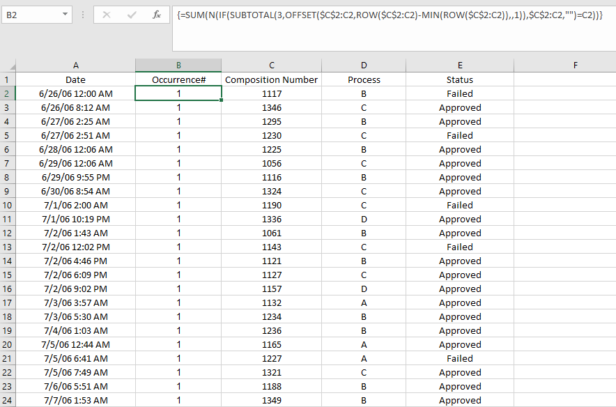
The array formula in the Occurrence# column is:
=SUM(N(IF(SUBTOTAL(3,OFFSET($C$2:C2,ROW($C$2:C2)-MIN(ROW($C$2:C2)),,1)),$C$2:C2,””)=C2))
Without going into a lot of detail on how this formula works, based on the selected Composition Number in column C, is uses an auto-expanding range that only produces a value of 1 if the rows are visible and then sums those instances. In this example, selecting only the compositional number 1127 produces the filtered table shown in the figure.

In the Process column, if A and B are removed through filtering, the result is:

Finally, if Approved is removed the Status column through filtering, the result is:

It is important to note that this formula is quite calculation-intensive. There are 5000 records in the example workbook, and it takes several seconds to recalculate after each filter change.
You can download the workbook here.