Using Conditional Formatting to Highlight Unique Items in an Excel Filtered List By David Hager

Quite a while back I created a formula to count the number of unique items in a filtered list. For examples, see:

http://blog.contextures.com/archives/2010/10/04/count-unique-items-in-excel-filtered-list/

and

https://dhexcel1.wordpress.com/2017/01/08/creating-a-unique-delimited-string-from-an-excel-filtered-list-by-using-the-textjoin-function-by-david-hager/

I decided to extend this methodology to the conditional formatting of a filtered list. The following defined name formulas are required.

Rge=$A$5:$A$29

unRge=IF(SUBTOTAL(3,OFFSET(Rge,ROW(Rge)-MIN(ROW(Rge)),,1)),Rge,””)

cfUnRge=INDEX((N(IF(ISNA(MATCH(“”,unRge,0)),MATCH(Rge,Rge,0),IF(MATCH(unRge,unRge,0)=MATCH(“”,unRge,0),0,MATCH(unRge,unRge,0)))=ROW(Rge)-MIN(ROW(Rge))+1)),ROW()-4)

(The cursor must be on A5 when the cf function is defined and applied to A5:A29)

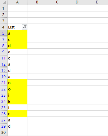
So, before filtering, the list shows the 1^st unique items highlighted in yellow.

After filtering (removing the letters b,e,f,g), the resulting filtered list looks like this.

I hope that this is another useful tool to add to your Excel bag of tricks. You can download the file from the link below. Enjoy!

unFiltered